Rising income inequality in the United States over the past several decades has been well documented in the economics literature.2 Recent studies have also looked at the dispersion in consumption, since it more accurately captures disparities in economic well-being. Here, however, the findings are mixed–while some authors find the dispersion in consumption has risen more slowly than that for income, others conclude that consumption inequality has closely followed the upward trends in income inequality.3 In this note, we assess the pattern of consumption inequality using an alternative data source–namely, new motor vehicle purchases. In short, when viewed from the lens of these direct spending data, we find little evidence that consumption inequality has risen as dramatically as income inequality over the past 15 years.
The existing literature generally has relied on surveys of spending, which offer a view of consumption trends through the analysis of numerous components of expenditure. We instead assesses the recent path of consumption inequality by looking specifically at data on new motor vehicle purchases. These data offer some advantages: First, our data cover the universe of registrations of new vehicles in the United States from the first quarter of 2002, with additional details on the county, the type of registration (commercial, government, rental, and retail), and the make and the model of the vehicle. The universal coverage of the dataset limits concerns regarding data quality.4 Second, our data are available at a quarterly frequency, and they are quite timely–estimates are available approximately 45 days after the quarter has ended. That said, an obvious limitation relative to earlier studies is the unit of analysis: with only county-level data, we must focus our analysis on trends in inequality across counties rather than individuals or households.5
In our analysis, we use model-level counts of vehicle registrations in each county that were recorded as “retail purchases”–a category that accounts for more than half of all registrations–and we merge these data with the 2016 manufacturer’s suggested retail prices (MSRPs) for each make and model to create county-level spending aggregates.6, 7 The heat map in figure 1 illustrates the geographic variation in average annual changes in these spending estimates among US counties between the first quarter of 2002 and the first quarter of 2017. The blue shaded areas indicate increases, while red-yellow shades represent declines. While the majority of counties recorded decreases, gains were concentrated in the Mountain States and the American South. McKenzie County, North Dakota, recorded the fastest growth of about 12 percent per year between 2002 and 2017; at the other end of the spectrum, Arthur County and Sioux County in Nebraska recorded the biggest declines.
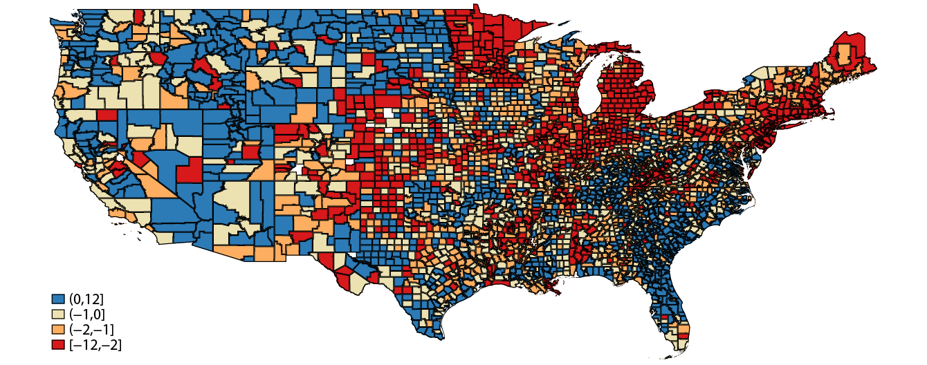
Note: Annualized changes in new vehicle registrations between 2002q1 and 2017q1.
Source: IHS Markit, new vehicle registration data.
To explore how our spending measure relates to the income distribution, we grouped all counties into three ranked bins based on their average personal income per capita between 1969 and 2000.8 By relying on income information from previous decades, our bin classification is less likely to be correlated with contemporaneous income shocks that might affect consumption. Figure 2 shows that the pattern of spending has varied substantially across counties in different terciles of the income distribution. Per capita vehicle purchases in top-income counties showed noticeable declines in 2005 and 2006, before the onset of the Great Recession. And while spending in top-income counties moved up again early in the recovery, it has since flattened out at levels well below the pre-recession peak. By contrast, counties in the middle and bottom income terciles registered smaller absolute declines during the Great Recession, and spending in these bins has almost completely recovered back toward pre-recession levels. As a result of these patterns, counties in the top income tercile account for about two-thirds of all registrations, but their share has slightly declined relative to 2002.
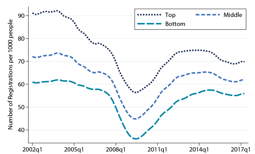
Note: Number of registrations is weighted by 2016 MSRP vehicle prices and deflated by new motor vehicle price index.
Source: IHS Markit.
Relative changes in the pattern of vehicle purchases across income groups have implications for the trends in consumption inequality. With differences between purchases for counties in the top income group and those in the bottom group shrinking over time, we would expect the overall cross-county dispersion in motor vehicle purchases to show a decline as well. The left panel of figure 3, which shows the cross-county dispersion of (log) vehicle consumption, confirms the qualitative patterns highlighted by figure 2.9 In particular, our measure of the dispersion in vehicle purchases dropped by about 5 percent (0.05 log points) between 2002 and 2011; thereafter, the dispersion began rising again, and by the beginning of 2017 it had moved up close to the levels observed early in the sample.
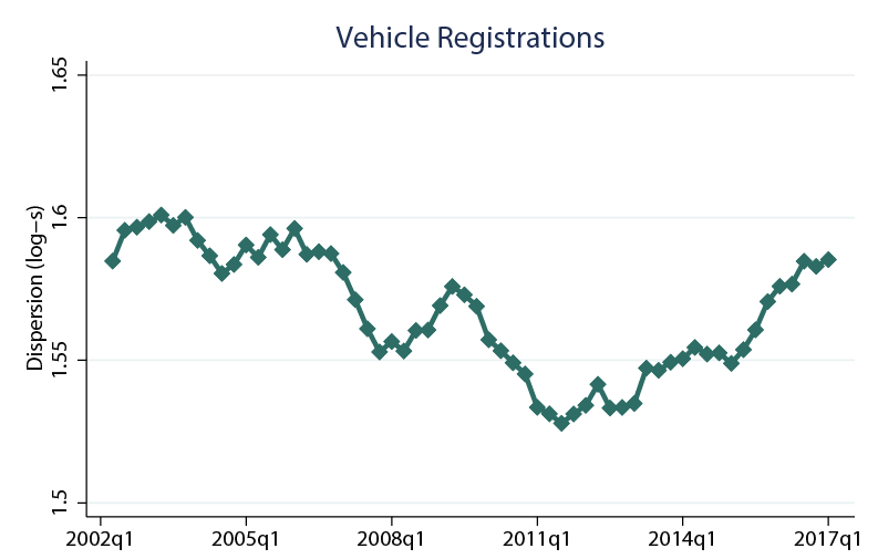
Note: Across-county dispersion in (log) vehicle registrations.
Source: IHS Markit.
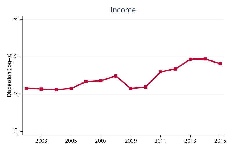
How does our measure of the dispersion in motor vehicle purchases relate to consumption inequality more broadly? If we assume an income elasticity of around two for vehicle purchases, a back-of-the-envelope calculation suggests that consumption inequality diminished by about 10 percent between 2002 and 2011 before moving back up near its initial level in 2016.10 For comparison, the right panel of figure 3 illustrates equivalent county-based estimates of per-capita income inequality. Income dispersion, by contrast, appears to have trended up steadily over the past 15 years. The pattern of rising income inequality over this time period is broadly consistent with the analysis of Aguiar and Bils (2015) and Attanasio, Hurst, and Pistaferri (2015).11
In an earlier study using household-level data, Kruger and Perri (2006) present evidence that consumption inequality rose less markedly than did income inequality over the 1983 to 2002 period. The authors also decomposed the trends in consumption and income inequality into the portions arising between vs. within groups of households with similar demographic characteristics; they conclude that while between-group consumption inequality roughly tracked the pattern of income inequality, within-group consumption inequality increased by much less than income inequality. Inspired by this analysis, we ran a similar exercise using our county-level data. For each year, we estimated a regression of the dispersion in consumption or income on a variety of demographic controls for each county, including population; the net migration rate; the age, sex, and race composition; the employment level; and the number of establishments.12 The residual sum of squares from these regressions thus represents the dispersion in income or consumption that cannot be explained by differences in observable county characteristics–or as Krueger and Perri (2006) refer to it, the within-group component of inequality. We find that the observable characteristics included in our regressions tend to explain a large share of the cross-sectional variation in both motor vehicle purchases and income (about 90 percent for motor vehicle purchases and 50 percent for personal income in 2002). Figure 4 depicts our estimates of within-group inequality for both income and consumption, where all estimates are indexed to zero in 2002.
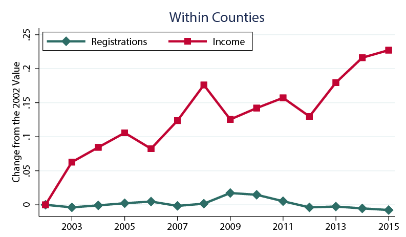
Note: Changes in residual within-county variation for registrations and income after controlling for demographics characteristics; 2002 values are normalized to zero.
Source: IHS Markit, Census, CBP, and BEA.
Similar to the Krueger and Perri (2006) results for the earlier time period, our data indicate that the within-group component has remained fairly constant for consumption inequality, even as it has risen substantially for income inequality. This finding is consistent with the idea that the increased income inequality owes at least partly to increased volatility of idiosyncratic income shocks.
Another factor that may have contributed to the recent trends in inequality is the transformation of the oil and gas industry during the co-called shale boom. During the early 2000s, technology advancements enabled large increases in drilling activity and oil production that then translated into income shocks–either in the form of labor compensation or through royalty payments to mineral rights owners–in the major shale-producing areas, such as the Permian basin and the Bakken region. If consumers viewed the income shocks arising from these developments as transitory, then they would be less likely to adjust their spending commensurate with the boost to income; and as such, the shale boom may partly account for the differing trends in consumption and income inequality in recent years. To gauge the importance of these effects, we added to our yearly regressions a dummy variable equal to one for those counties in areas with shale formations, as classified by the Energy Information Administration. We find that the addition of this dummy variable helps explain about 0.1 percentage point of the between-group dispersion in income, but it does not enter significantly in the equation for the dispersion in consumption.13 We leave a deeper exploration into the implications of oil and gas developments for income and consumption inequality for future research.
References
Aguiar, Mark, and Mark Bils (2015). “Has Consumption Inequality Mirrored Income Inequality?” The American Economic Review, vol. 105(9), pp. 2725-2756.
Attanasio, Orazio, Erik Hurst, and Luigi Pistaferri (2014). “The Evolution of Income, Consumption, and Leisure Inequality in the United States, 1980–2010,” in Christopher D. Carroll, Thomas F. Crossley, and John Sabelhaus, editors, “Improving the Measurement of Consumer Expenditures” University of Chicago Press.
Attanasio, Orazio P., and Luigi Pistaferri (2016). “Consumption inequality.” The Journal of Economic Perspectives 30(2), pp. 3-28.
Battistin, Erich (2003). “Errors in Survey Reports of Consumption Expenditures.” IFS Working Papers No. 03/07, Institute for Fiscal Studies (IFS).
Bordley, Robert F., and James B. McDonald (1993). “Estimating Aggregate Automotive Income Elasticities from the Population Income-Share Elasticity,” Journal of Business and Economic Statistics, vol. 11, pp. 209-214.
Bricker, Jesse, Rodney Ramcharan, and Jacob Krimmel (2014). “Signaling status: The impact of relative income on household consumption and financial decisions.” Finance and Economics Discussion Series 2014-76.
Brown, Jason P. (2017). “Response of Consumer Debt to Income Shocks: The Case of Energy Booms and Busts.” The Federal Reserve Bank of Kansas City Research Working Papers 17-05, available at https://doi.org/10.18651/RWP2017-05.
Garner, Thesai, George Janini, William Passero, Laura Paszkiewicz, and Mark Vendemia (2006). “The Consumer Expenditure Survey: A Comparison with Personal Expenditures,” Bureau of Labor Statistics.
Krueger, Dirk, and Fabrizio Perri (2006). “Does Income Inequality Lead to Consumption Inequality? Evidence and Theory.” The Review of Economic Studies, vol. 73(1), pp. 163-193.
Levy, F., and R. J. Murnane (1992). “U.S. Earnings Levels and Earnings Inequality: A Review of Recent Trends and Proposed Explanations.” Journal of Economic Literature, vol. 30, pp. 1333–1381.
McCarthy, Patrick S. (1996). “Market Price and Income Elasticities of New Vehicle Demands.” The Review of Economics and Statistics, pp. 543-547.
Piketty, Thomas, and Emmanuel Saez (2003). “Income Inequality in the United States, 1913–1998.” Quarterly Journal of Economics, vol. 118(1), pp. 1-41.
1. We thank James Calello for excellent research assistance. The views expressed in the article are those of the authors and do not necessarily reflect those of the Federal Reserve System. Return to text
2. See, among others, Levy and Murnane (1992); Piketty and Saez (2003); Attanasio, Hurst, and Pistaferri (2015); and Attanasio and Pistaferri (2016). Return to text
3. See Aguiar and Bils (2015) and Attanasio, Hurst, and Pistaferri (2015). Return to text
4. Many papers (see, among others, Battistin, 2003; Garner et al., 2006) have documented systematic measurement errors on consumption growth in the Consumer Expenditure Survey, a widely used source to analyze consumption inequality. Return to text
5. IHS Markit also collects registration data at the zipcode level, but we have access only to data from the period 2006:Q1 to 2010:Q4, with no information on make or model. Return to text
6. The new vehicle registration data also include consumer leases. Extending our analysis to all consumer transaction–i.e., retail purchases and leases–does not significantly alter our results. Return to text
7. Using relative vehicle prices ensures that our measures capture different cross-county trends towards luxury brands, as those are important to evaluate overall inequality. See, for example, Bricker, Ramcharan, and Krimmel (2014). Return to text
8. Estimates of personal income are from the Bureau of Economic Analysis (BEA) and are defined as the sum of wages and salaries, including employer contributions to pension funds; current transfer receipts; entrepreneurial withdrawals; and dividends, interest, net rents, and royalties. Per capita personal income is then calculated as the personal income of the residents of a given area divided by the resident population of that area. Return to text
9. Our measures of inequality are influenced by differences in cross-county characteristics, such as population and age composition, migration patterns, trends in urban vs. rural areas, distribution of income, etc. Our decomposition into between- and within-county components of consumption and income inequality aims at controlling for some of those differences. Return to text
10. Existing empirical estimates of income elasticities from time-series studies have generally ranged around 2. Bordley and McDonald (1993) report an income elasticity of vehicle demand of 2.1, while McCarthy (1996) estimates that after controlling for vehicle quality, the elasticity of demand is 1.7. Return to text
11. Aguiar and Bils (2015) find that income inequality, measured as the ratio between the 95th-80th and 5th-20th percentile, increased 2 log points in before-tax income between 2005-07 and 2008-10; Attanasio, Hurst, and Pistaferri (2015) estimate that the standard deviation of log before-tax income increased by about 0.07 log points between 2000 and 2010. Return to text
12. Data on the employment level and the number of establishments are from the Census Bureau’s County Business Patterns; data on population characteristics are from the Census Bureau’s Population Unit Estimates. The age composition exploits all age groups above 14 years of age in 5 year bins (we aggregated in a single group all people above 64). The race composition includes controls for the share of white only and black only. Return to text
13. Brown (2017) also presents evidence to support the idea that consumers tend to view oil price shocks as transitory. In particular, the author documents that while consumers are willing to increase their spending following an energy-driven income shock, they require 5 percent more drilling activity to trigger the same response in auto debt as in other consumer debt. Return to text
Disclaimer: FEDS Notes are articles in which Board economists offer their own views and present analysis on a range of topics in economics and finance. These articles are shorter and less technically oriented than FEDS Working Papers.